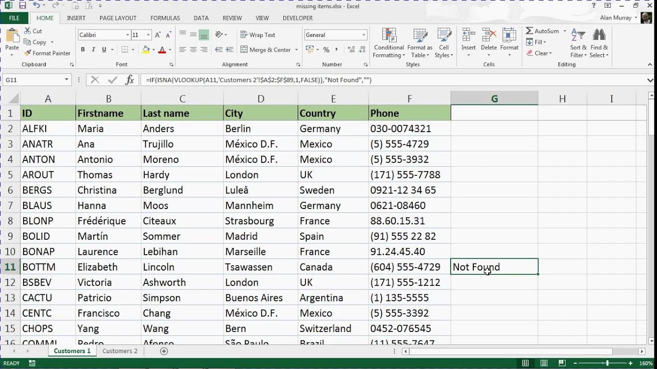
How To Do A Vlookup In Excel To Find Missing Data
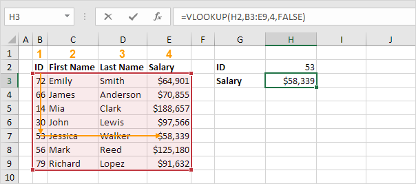
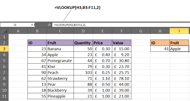
33 rows For VLOOKUP this first argument is the value that you want to find. In the example shown the formula in G6 is.
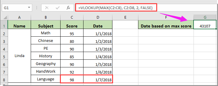
How To Vlookup And Return Date Format Instead Of Number In Excel
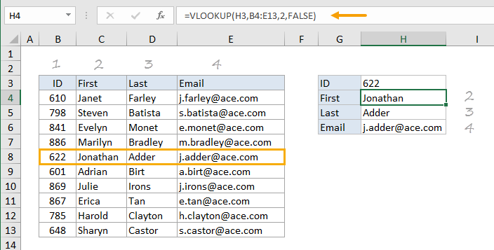
Lookup_value Find the Unique Identifier lookup value.

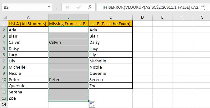
How to do a vlookup in excel to find missing data. We will construct a formula out of it. Select the first blank cell besides Fruit List 2 type Missing in Fruit List 1 as column header next enter the formula IF ISERROR VLOOKUP A2Fruit List 1A2A221FALSEA2 into the second blank cell and drag the Fill Handle to the range as you need. Table_array - the data range in the lookup sheets.
Lookup_value - the value to search for. And then the returned value passed into LEN function as it argument. It is usually in the same row as the empty cell you selected.
At the top go to the Formulas tab and click Lookup Reference. Lookup_range - the column range in the lookup sheets where to search for the lookup value. Open the VLOOKUP function first.
In its simplest form the VLOOKUP function says. Excels vLookup wizard will pop up. Click Home in ribbon click Conditional Formatting in Styles group.
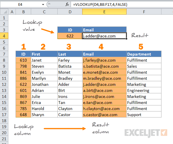
The function looks for the lookup_value in the first column of the data table. The COUNTIF statement returns the results which play a role as the first argument of IF statement for the logical test to be performed. To find the missing values from a list define the value to check for and the list to be checked inside a COUNTIF statement.
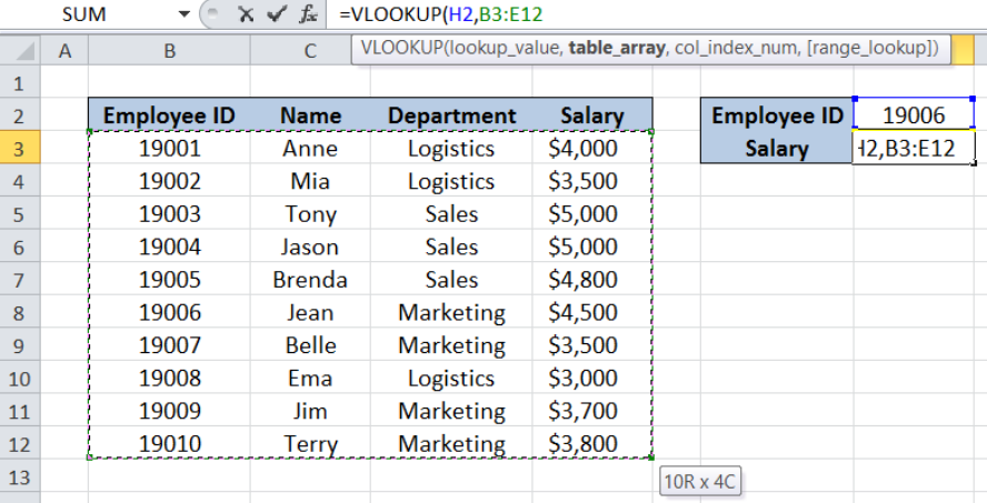
IFVLOOKUPE5 data20 VLOOKUPE5 data20. Out lookup value will be the C2 cell value because we are comparing List A contains all the List B values or not so choose C2 cell reference Cell Reference Cell. This argument can be a cell.
VLOOKUP What you want to look up where you want to look for it the column number in the range containing the value to return return an Approximate or Exact match indicated as 1TRUE or 0FALSE. Col_index_num - the number of the column in the table array from which to return a value. How to compare data in two columns to find duplicates.
The first VLOOKUP formula will lookup value excel in range A1B5 if TRUE then return the corresponding value in Column B. The VLOOKUP function uses the following arguments. Compare Two Columns to Find Missing Value by Conditional Formatting.
Firstly the lookup value is searched in the particular column of the table array. The Len function will return the length of the returned value by VLOOKUP Function. Table_array required argument The table array is the data array that is to be searched.
Then the matched values will give us the confirmation using the IF function. In the image above example this is table B5F17 and this range is the table_array argument. Select List A and List B.
You supply the column number as the col_index_num argument which tells VLOOKUP which column contains the data you seek. To identify values in one list that are missing in another list you can use a simple formula based on the COUNTIF function with the IF function. Lookup_value required argument Lookup_value specifies the value that we want to look up in the first column of a table.
You provide a name or lookup_value that tells VLOOKUP which row of the data table to look for the desired data. If the value is found in the list then the COUNTIF statement returns the numerical value which represents the number of times the value occurs in that list. To do this select File Options Customize Ribbon and then select the Developer tab in the customization box on the right-sideClick Find_Matches and then click RunThe duplicate numbers are displayed in column B.
Locate where you want the data to go. In the example shown the formula in G5 copied down is. IFCOUNTIF list F6 OKMissing where list is the named range B6B11.
In Conditional Formatting dropdown list select Highlight Cells Rules-Duplicate Values. The matching numbers will be put next to the first column as illustrated here. The second step is to select the data where this info is available.
Click that cell only once. The IF function returns the confirmation using the values Is there Missing. Summary To check for empty cells in VLOOKUP results you can combine the VLOOKUP function with the IF function.
Since you can spend a long time analyzing and finding the required information Excels VLOOKUP function was created to simplify data retrieval. VLOOKUP performs the search in the first column and retrieves the info from whichever column you specify to the right. VLOOKUP works by performing a vertical search top.
Well walk through each part of the formula.
How To Use The Excel Vlookup Function Exceljet
![]()
How To Vlookup To Return Blank Or Specific Value Instead Of 0 Or N A In Excel
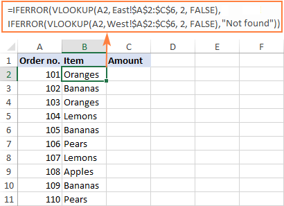
Vlookup Across Multiple Sheets In Excel With Examples
Excel Formula Faster Vlookup With 2 Vlookups Exceljet
Compare Two Lists Using The Vlookup Formula Youtube

Excel Formula Vlookup Without N A Error Exceljet

Excel Vlookup With Missing Data Super User
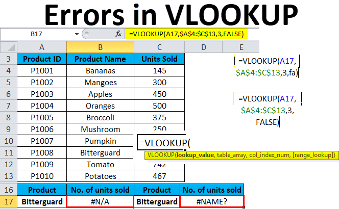
Vlookup Errors Examples How To Fix Errors In Vlookup
How To Use The Excel Vlookup Function Exceljet

Vlookup Missing Items Exercise See Solution Link Below How To Find Missing Items With Vlookup Youtube
Excel Vlookup The Ultimate Guide To Mastery


Find Missing Values In Excel
Vlookup With Table Array 5 Best Practices Excelchat
How To Use The Excel Vlookup Function Exceljet
![]()
How To Vlookup To Return Blank Or Specific Value Instead Of 0 Or N A In Excel
How To Use The Excel Vlookup Function Exceljet
How To Compare Two Columns To Find Missing Value Unique Value In Excel Free Excel Tutorial
6 Reasons Why Your Vlookup Is Not Working
Vlookup Examples In Excel September 5 2021 Excel Office